In this issue, we’d like to introduce a powerful new feature of the STEP SPad teach pendant: its data acquisition function. Similar to the trace function in CODESYS, this feature enables data configuration and acquisition directly on the teach pendant. The acquired data can be displayed as 2D curves, and you can perform various operations on these curves, such as single-channel or multi-channel display, dragging, zooming in and out, and adding cursors—making it easier to conduct further data analysis.

Data Acquisition Interface

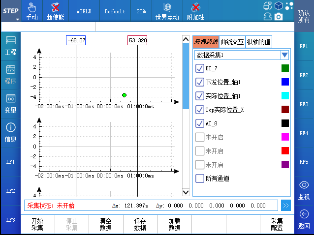
Click STEP > Advanced Monitoring > Data Collection to enter the data collection interface, as shown in the figure below:

Collection Configuration

Click the Collection Configuration button in the lower-right corner of the data collection interface to enter the collection configuration interface. By default, there are four collection configurations—Data Collection 1 through Data Collection 4. Each data collection group consists of three parts: basic configuration, trigger method configuration, and channel configuration.

The collection configuration interface is shown in the figure below:

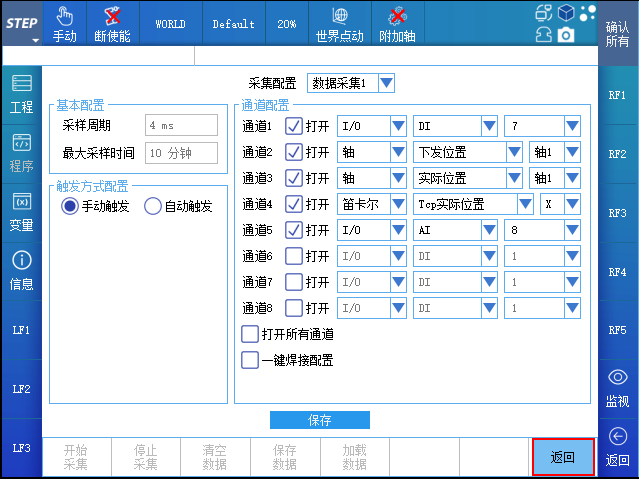
Basic configuration Includes the sampling period and the maximum sampling time. The default sampling period is 4 ms, and the default maximum sampling time is 10 minutes; neither requires user configuration.

Trigger method package It supports both manual and automatic triggering. For manual triggering, no trigger configuration is required—simply click the “Start Acquisition” button to initiate data acquisition. For automatic triggering, a trigger must be configured first; data acquisition will only begin once the trigger is activated. There are two types of triggers used in automatic triggering: ❶ Start Motion: Data acquisition is triggered only when the robot starts moving; ❷ DI/DO: Data acquisition is triggered only after a signal is detected, with the signal distinguished by rising and falling edges.

Channel Configuration By default, there are 8 channels available. You can configure the data to be collected on each channel and specify whether a channel is enabled. Data collection for a particular channel becomes possible only after the channel has been enabled. For example, when configuring data collection 1, you can enable Channel 2 and set the data for Channel 2 as “the downstream position of Axis 1.”

After you have configured the trigger method and channel settings, simply click the Save button to save your changes.

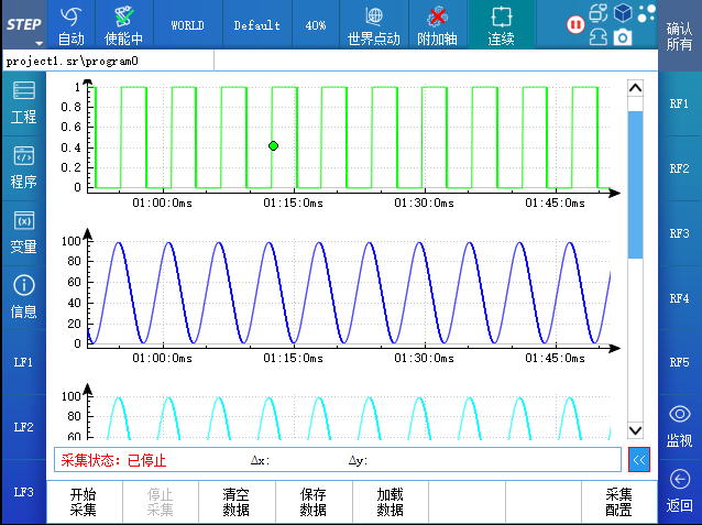
Data collection operation

On the data acquisition interface, select a configuration set from Data Acquisition 1 to Data Acquisition 4 to view the contents of Channels 1 through 8 corresponding to that configuration set. If the acquisition is manually triggered, you can immediately see the real-time 2D curve of the acquired data after clicking Start Acquisition. If the acquisition is automatically triggered, you can view the 2D curve of the acquired data after clicking Start Acquisition and waiting for the trigger to be activated. Meanwhile, the current acquisition status is displayed in the status indicator, which can be one of four states: Not Started, Waiting for Trigger, Acquiring, or Stopped.

Click the Stop Collection button to stop collection, or the system will automatically stop collection once the maximum collection time is reached. When stopping collection, you can select the checkbox corresponding to each channel on the right to specify whether to display the corresponding curve.

The above operation is shown in the figure below:

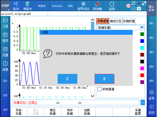
The software can simultaneously cache the collected data corresponding to Data Acquisition 1 through Data Acquisition 4. When you click the "Clear Data" button, all cached data associated with Data Acquisition 1 through Data Acquisition 4 will be cleared. After the data is cleared, the corresponding 2D curves will no longer be displayed on the interface. Additionally, when you click "Start Acquisition," the cached data for the currently selected data acquisition will be automatically cleared. Clearing the data frees up memory, which helps improve the software's running speed.

The data clearing interface is shown in the figure below:

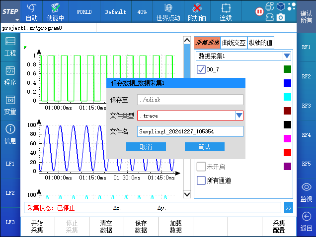
Saving data allows you to save the current data acquisition information into a file on a USB drive. Loading data enables you to load the data from the USB drive onto the teach pendant and display it in the form of a 2D curve. The file formats for saving and loading data can be .trace or .csv.

The data saving interface is shown in the figure below:

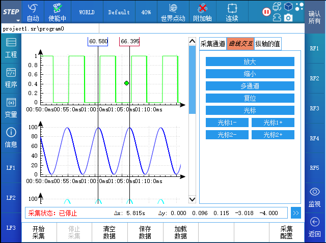
Curve interaction operation

After data acquisition has been stopped or after external data has been loaded from a USB drive, you can analyze the data through interactive 2D curve operations. For example, clicking the zoom-in button will zoom in on the curve centered around the current cursor position; clicking the zoom-out button will zoom out on the curve, again centered around the current cursor position; and clicking the reset button will restore all curves to their original view within the visible area. The current cursor position is indicated on the interface by a green dot, and the position of this dot will change as the user touches the screen.

The above operation is shown in the figure below:

A single data acquisition can collect up to 8 sets of data. When multiple sets of data are displayed on the same graph, you can choose to show all curves in a single coordinate system (single-channel mode) or display each curve in its own separate coordinate system (multi-channel mode).

The default is multi-channel display, which is shown in the figure below:

When displaying in multi-channel mode, click the “Multi-channel” button to switch to single-channel display, as shown in the figure below:

To facilitate data analysis, you can click the cursor button to insert one or two cursors. You can simultaneously view the X-axis values of all curves corresponding to each cursor, as well as the X- and Y-axis differences between the curves within the range defined by the two cursors. By dragging the rectangular box above the cursor left or right, you can move the cursor horizontally. As you move the cursor, the corresponding X-axis value and the X- and Y-axis differences will update accordingly. You can also fine-tune the cursor’s position by moving it slightly left or right; during fine adjustments, the cursor moves in increments of 2 milliseconds each time.

The cursor interaction is shown in the figure below:

Shortcut key function

Click STEP > Control Panel > Buttons & Keys to enter the shortcut key configuration interface, as shown in the figure below:

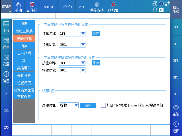
On this interface, you can configure the shortcut key functions for LF1-LF3 on the left side of the teach pendant screen, RF1-RF5 on the right side, and the hardware buttons KeyF1-KeyF4 on the teach pendant. Click the drop-down list to select the corresponding function, then click Save, and the shortcut keys will take effect immediately.

The “Robot Classroom” series of articles is designed to truly help those of you who are currently operating and using STEP robots. If you have any questions about the operation or use of STEP robots, feel free to interact with us on the message board or give us a call at our customer service hotline. See you in our next episode!

Email:
market@stepelectric.com

Address:
No. 1560, Siyi Road, Jiading District, Shanghai Municipality